An article by Maurice Gilroy in a recent issue of Reciprocity1 clearly brings to focus the fact that more fundamental theoretical work needs to be done on the rotational motions of atoms. Few years ago, studying the electric ionization characteristics of the elements in the context of the Reciprocal System, I had come to the same conclusion with regard to the non-conformist nature of the lanthanides. Presently I have made a more detailed examination of the mathematical structure of the scalar rotational motion with a view to obtain some insight into these fundamentals. I am reporting in this Paper the results of this study. My conclusions, as yet, are by no means final. However, it is felt desirable, in view of the maiden nature of the exploration, to invite comments and discussion before bestowing further efforts on it.
1 Introduction
The basic features of scalar rotational motion that constitutes atoms are described in Chapters 9 and 10 of Larson's book, Nothing But Motion.2 The rotation that is basic to the material atoms is a two-dimensional rotation, involving a coupled rotation about two, mutually perpendicular axes (in the three-dimensional time). Larson reminds us in this connection that “…there are not two one-dimensional rotations; there is one two-dimensional rotation… The combined magnitude of two one-dimensional rotations of n displacements each is 2n. The magnitude of a two-dimensional rotation in which the displacement is n in each dimension is n2.”3 Before passing further it is to be noted that this is true only for a spherically distributed two-dimensional rotation. On the other hand, if the two dimensions are unequal, say, m and n the rotation is distributed in the form of a spheroid and its magnitude would be neither n nor m but m×n.
Larson adopts a notation of the form a b c to designate the various rotations involved, with “… c …[as]… the displacement of the one-dimensional reverse rotation, and a and b … the displacements in the two dimensions of the basic two-dimensional rotation.”4 A little later he demonstrates that “… a magnetic displacement n is equivalent to 2n2 electric displacement units.”5 At this juncture a question arises. Suppose the respective displacements in a certain case are given by a b c. The electric equivalents of the magnet displacements a and b are calculated, according to Larson, as being 2a2 and 2b2 respectively. This means only one thing: that a and b represent two separate spherically distributed two-dimensional displacements—they are not, as Larson describes in the above cited quotation,4 the displacements in the two dimensions of the basic two-dimensional rotation.
Because if the latter is true they ought to represent a spheroidally distributed rotation with magnitude equivalent to 2×a×b electric displacement units (see Appendix). This, therefore, is a point that needs to be straightened out.
A second factor I wish to comment upon is regarding the way the successive increments in the magnetic rotations takes place. Unlike in the case of electric displacement the increment in the magnetic displacement is not one by one. The first increment in the magnetic displacement is 2×12 = 2 electric units long. The second increment, however, is 2×22 = 8 electric units long. It is quite understandable, in view of the 2n2 relation between the magnetic and electric units, why there can be, for example, no such thing as a magnetic equivalent of 6 electric units (since $\sqrt{6/2}$ is not an integer) and consequently the 8 (= 2×22 ) units do not represent the total after the second increment but the second increment itself—the total being 10 (= 2+8). But this does not explain why 2×22 = 8 units should succeed 2×1 = 2 units; why not the successive increments be of 2×1 units size each (since $\sqrt{2/2}$ is an integer). Here too, a further theoretical clarification of the fact that the successive increments of the magnetic displacement are of 2, 8, 18 and 32 electric unit equivalent is in order.
2 The Mathematical Pattern of the Two-Dimensional Rotation
The most important factors that are relevant to our present study can be listed as follows:
-
Motion occurs in discrete units.
-
A smaller number of displacement units are relatively more probable than a larger number of them.
-
The scalar rotation which constitutes the atom takes place inside unit space (the “time region,” as it is called).
Before we begin the discussion, perhaps a word of caution is in order. We often find the insights and conclusions obtained through the Reciprocal System queer and bizarre. This is only because, despite repeated admonitions, we continue to look at them from a frame of thought based essentially on the matter concept of the universe and not on the motion concept. Nothing impedes progress in the study of the Reciprocal System more than the inability to look at the new concepts on their own right.
2.1 Successive Increments of Displacement.
We begin our discussion by a consideration of the time region, the region inside unit space. Because of the discrete unit postulate, we see that in the time region, space can not progress on its own right and is constant at one unit. Therefore, Larson points out, “… The additions in the time region follow a different mathematical pattern, because in this case only one of the components of motion progresses, the other remaining fixed at the unit value. Here … the sequence is 1/1, 1/2, 1/3 ... 1/n. The quantity 1/n is the final term, not the total.”6
This requires certain elucidation. We recall that all units of space (or time) are alike, since each is equivalent to n unit of time (or space). “Alike” strictly means indistinguishable from each other. Normally, when two entities are alike in all respects we, nonetheless, can distinguish them by position in three-dimensional space. The two entities, if they happen to occupy different units of space, can be distinguished by means of these different locations. However, when the entities under consideration are the units of space themselves, there is prima facie no way of distinguishing between them. Since space can not be a background or “setting” to itself, the possibility of discriminating by virtue of the occupancy of different locations in space does not exist in this case. The full implication of the identity of all space units, together with the repudiation of the "setting" concept is that we are not justified in conceiving of the juxtaposing of two single units of space, and consequently can never get started beyond the one unit space (or time) magnitude.
I can foresee that the point I am trying to make above might not readily be apprehensible and rather look like denying the obvious. But this would be so only because of the subtle conceptual impasse (a result of our mental vantage point) that naturally besets any endeavor to understand the unmanifest from the standpoint of the manifest. The fact is that when we commence our inquiry (of the basic space unit), we already start with the conceptual background of an extension space in which we picture one unit of space “adjacent” to another unit of space. This, of course, is the fatal mistake that had been perpetrated by all the previous scientific thinkers and laymen, as Larson points out.7
Considerations like the above lead us to the conclusion that each succeeding space unit or increment has got to be one unit greater in magnitude than the previous. That is, the first increment is of one unit magnitude, the second increment is of two units magnitude and so on. This, of course, follows from the fact that the progression is continuous and ubiquitous. Thus if we consider a line segment AB as the given unit of space, it is not legitimate to envision the progression as the growing of this line AB to ABC, with the original segment AB intact and BC as the newly added portion. In reality there is growth at every point of the segment, with AC supplanting AB.
Further, we note: (i) there is no space progression divorced from a concomitant time progression and (ii) an increase in time magnitude is equivalent to a decrease in space magnitude. Suppose if we take A to be the reference point, then it becomes the starting point and B the ending point of the first space unit AB. However, since the progression of time nullifies the progression of space, the ending point in space-time always coincides with the starting point and point A will be the starting point from which the second unit (increment) of space “extends.” Thus AC becomes the second space unit and not BC. Though the second unit (AC) is of two units magnitude, since the first (AB) has been supplanted, the total up to the end of the second is also two units and there is an effective increment of only one unit (BC).
Inside the time region (or space region) too this process is the same: namely, the first increment is of one unit magnitude, the second increment is of two units magnitude and so on. However, in this region only one of the components of motion (either time or space) progresses. Consequently, the situation of the progression of one component getting nullified (from the point of view of space-time) by the progression of the reciprocal component does not occur and the starting point of the next increment is not the same as the starting point of the earlier increment, as it was in the outside region. Instead, the ending point of the previous increment will be the starting point, of the next.
Summarizing: in the outside region where both components of motion progress, the successive increments would be 1, 2, 3, 4… etc., though the successive effective increments would be
|
2-1, 3-2, 4-3, ...etc. |
(1) |
This is the same thing as saying that there is first one effective unit increment followed by another effective unit increment and so on and on. In a similar fashion, the successive increments in the time region (or the space region) would be
|
1, 2, 3, 4, ...etc. |
(2) |
(What the successive effective increments would be will be discussed in a moment.) Thus the nth increment of the displacement is n units in magnitude. The corresponding successive increments of the speed (above the neutral point of one unit) are 2, 3, 4, 5… etc. in the case of space displacement, and 1/2, 1/3, 1/4, 1/5,… etc. in the case of time displacement. It may be added that the above is true irrespective of whether the displacement is one-dimensional or two-dimensional. The pattern of increments indicated in (2) above, doubtless, looks quite unfamiliar. The fact is that this has not been found earlier as nobody knew about the time region before the advent of the Reciprocal System.
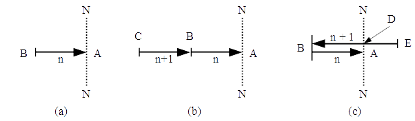
The next point of crucial importance that emerged in the investigation was the result of operation of the probability principle mentioned at the beginning of this section. Referring to Figure 1(a), let BA represent n displacement units, shown to the left of the neutral axis NN, but extending toward NN. NN represents the “zero-datum” of the natural reference system, which is unity. As such, BA represents a displacement of n units toward unity, that is, an inward scalar speed. In Figure 1(b) is shown what could be the result of adding the next increment of the displacement which, by conclusion (2) above, has to be n + 1 units in magnitude, bringing the total to 2n + 1 units. However, the state of affairs depicted in Figure 1(b) never obtains for the following reason. At point B, where the previous increment, comes to an end, an option is open to the next increment either to continue the previous direction (as in Figure 1(b)) or to reverse it as shown in Figure 1(c). In the latter case, like in the former, there is a continuity between both the incremental stretches. In the case shown in Figure 1(c), whose the next increment of n+1 units extends from E to B, the orientation of the displacement is still inward (that is, toward NN) from E to D, whereas it is outward for the portion from D to B. Since the latter portion (DB) coincides with the outward (away from NN) scalar progression of space-time, it is not effective from the point of view of physical phenomena. Consequently, the effective displacement is from E to D only. Since the orientation shown in Figure 1(c) ensues in a net displacement of smaller magnitude than that shown in Figure 1(b), the probability principles ensure that only the former exists in practice.
At this juncture I find it desirable to introduce certain new terminology both to facilitate further discussion and to help avoid bringing old frame of thinking into the now situation. Since it is now apparent that each further increment of the displacement reverses the direction of the previous orientation I shall refer to these increments as folds. Thus, in Figure 1(c), BA represents a fold and EB the next fold with ED as the effective portion of the second fold.
Summarizing our findings so far we can say that (i) each successive fold reverses its direction while maintaining continuity with the previous, and (ii) the nth fold is of n displacement units magnitude.
2.2 The Two-Dimensional Displacement
With the benefit of the above discussion, we are in a position to examine the pattern of the successive increments of the two-dimensional rotational displacement on which the atom structure is based.
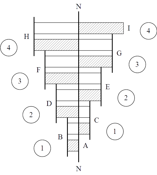
Referring to Figure 2, we have the first fold BA of one displacement unit magnitude. The arrows indicating the scalar direction are omitted: but it must be understood that the direction of the unit is always inward, that is, toward the neutral axis NN like in Figure 1.
The second fold is two units in magnitude and extends from C to B. However, only one unit of this fold is effective, the other being ineffective as its direction coincides with that of the background space-time progression. The effective portion of the fold is shown hatched in the figure. The magnitude (in number of displacement units) of the effective portion is shown circled adjacent to the hatched side of the rectangle representing the fold.
The third fold is of three units magnitude and extends from D to C. In this case the effective displacement is of two units magnitude.
Continuing the pattern we find on the seventh and the eighth folds (HG and IH respectively) a net (effective) displacement value of four magnetic units each. This brings the displacement value to the maximum that is possible for a two-dimensional rotation.8
Thus, though the successive folds are of magnitudes 1, 2, 3, 4, 5, 6, 7 & 8, the order of the effective increments is 1, 1, 2, 2, 3, 3, 4 & 4 units. Converting the magnetic units into the equivalent electric displacement units by the 2n2 relation, we now see that the possible series of successive increments of the two-dimensional rotational displacement has to be
|
2, 2, 8, 8, 18, 18, 32 & 32 units in magnitude |
(3) |
The magnetic displacement units we .are talking of, it may be reminded, are double magnetic units since we are considering them in connection with the double rotating systems of the atom (see Appendix). As such they represent the magnetic contribution of both the rotating systems. Therefore, in the notation a b c, a or b (respectively 2a2 or 2b2 electric displacement units) represents the motion on the two dimensions of the two-dimensional rotation of both the rotating systems. It is not that a represents the displacement on one dimension and b that on the other, of the two-dimensional rotation.
The necessity of two parameters, a and b, follows from another reason. We have seen that the successive folds of the two-dimensional rotation are in mutually opposite directions when seen from the point of view of the stationary reference frame, although their scalar direction relative to the datum of the natural reference system is always inward. Since rotation is a continuous motion, there is no possibility of representing these direction reversals as oscillations of a vibration in the stationary reference system. Therefore, the representation in the stationary reference system of the true scalar relationship between the successive folds takes the shape of interpreting the effective portions of the alternate folds (which are co-parallel) as belonging to a separate two-dimensional rotation. The sets of alternate folds, one on each side of NN, therefore, are depicted as belonging to different two-dimensional rotation, a and b in the notation a b c.
It must further be noted that neither a nor b represents the entire motion in that dimension of time but each gives only the magnitude of the largest fold of that motion. If we identify the effective magnetic displacements 1, 2, 3 and 4 indicated on the right side of NN with the dimension represented by a, the increments 1, 2, 3 and 4 shown on the left side of NN are to be identified with the dimension represented by b. Considering that there is an initial magnetic unit in one of the dimensions, say that of a, which is utilized to equilibrate the negative displacement of the basic photon, we see that the successive values taken up by a are 2, 3, 4 and 5 while those taken up by b are 1, 2, 3 and 4.
It will be of interest to note that the following behavior patterns directly result from the fold structure of the atomic rotational displacement:
-
Firstly, the effective displacement magnitude of each fold is able to act independently. This is the reason, why the calculation of the net total equivalent displacement, in any instance, proceeds as
|
$2 \times 1^2 + 2 \times 2^2 + 2 \times 2^2 + 2 \times 3^2 ...$ |
(4) |
but not as
$2 \left(1 + 2 + 2 + 3 ... \right )^2$
-
Because of the above, in many of the atomic interactions only the final fold (I wish to avoid calling it the “topmost”) with the largest magnitude in each dimension, is alone able to enter into relationship. (Examples occur in the determination of the interatomic distances, the ionization potentials etc.)
-
Also because of item (i) above, the limitation of the 4-unit maximum for the two-dimensional rotation applies to the individual folds and not to the net total. Were it not the case, the theoretically possible number of elements would turn out to be far less than 117.
3 The Mathematical Pattern of the Electric Displacement
With the exception of the modifications introduced by the characteristics of the one-dimensional rotation, the general pattern of the successive increments (folds) of the displacement in the electric dimension (represented by c in the notation a b c) is the same as in the case of the two-dimensional rotation.
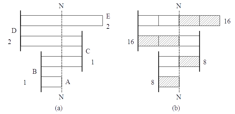
Figure 3(a) depicts this situation. First there is a one-unit increment BA; then there is the second fold CB, of 2-unit magnitude, with an effective magnitude of one unit and so on.
The important point that we should now recognize is that, in the context of the one-dimensional rotation, one unit really represents eight possibilities or degrees of freedom (see Footnote 8). Consequently, for all practical purposes we can treat this one “unit” as comprising eight electric displacement units. This results in the increment pattern depicted in Figure 3(b).
However, there is another possibility that is available to the one-dimensional electric displacement units by virtue of which the pattern depicted in Figure 3(b) gets modified. The eight unit limitation, it may be recalled, on the one-dimensional rotation was arrived at on the basis of three-dimensional distribution in the time region.8 But if the number of one-dimensional units is not more than two, they could be distributed either one-dimensionally or three-dimensionally. Consequently, the first fold in the increment pattern of the one-dimensional rotational displacement would be of two electric displacement units magnitude as shown by BA in Figure 4(a), and not of eight units magnitude as depicted in Figure 3(b). At this point the limitation of distribution on the one-dimensional basis is reached and the subsequent units of electric displacement will have to be added on the basis of three-dimensional distribution. The second fold, of eight electric displacement units magnitude, reverses the relative direction, as indicated by CB in Figure 4(a). It may be noted that the effective portion of the second fold is only of six units magnitude.
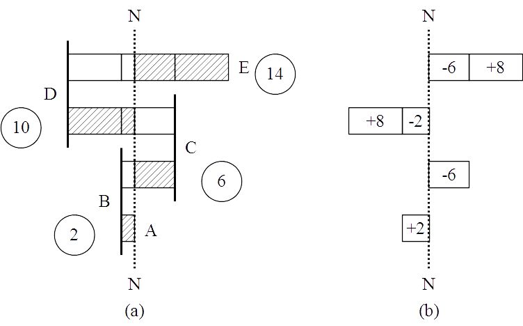
The third fold is of two 8-unit increments in magnitude, extending from D to C (Figure 4(a)). The effective portion, however, is only of ten electric units magnitude. In a similar manner, the effective magnitude of the fourth fold can be seen to be of fourteen electric units. The successive folds of the one-dimensional rotation, therefore, form the series
|
2, 6, 10 & 14 electric displacement units |
(5) |
We may pause here to comment that those who have wondered at the similarity between the 2n2 relation of the magnetic and electric displacement units of the Reciprocal System and the 2n2 relation of the “principal quantum number” of a “shell” and the maximum number of “electrons” the “shell” is supposed to hold in the matter-concept of the universe, would not have failed to notice the similarity between the series 2, 6, 10, 14 of the electric displacement units of the Reciprocal System and the “electron capacities” of the “s, p, d, f subshells” of the matter-concept theory! But I believe that the similarity ends there. For, the further possibility in the case of the one-dimensional rotation of the atoms that the electric displacement could be either positive (time-displacement) or negative (space-displacement) modifies the pattern of the folds in another way.
It is seen that the folds subsequent to the first, in the case of the one-dimensional rotation, are in stretches of multiples of eight units. At the end of an 8-unit stretch, there opens up before the rotation a possibility to switch from a positive displacement to a negative displacement or vice versa. This would be tantamount to the effect of reversing the relative direction that occurs when one fold ends and the next one begins. The probability principles indeed favor this switching as it reduces the net effective magnitude of a fold. The actual pattern of the successive increments of the one-dimensional rotation of the atom is therefore as shown in Figure 4(b).
We have two positive electric displacement units in the first fold. The second fold is really the continuation of the first fold as the three-dimensional limit of eight units is not yet reached. As such, it is to be expected that the first fold should continue up to eight units magnitude instead of the two. Indeed this would have been the case but for the additional possibility that is available to the electric displacement, namely, to switch from the positive to the negative displacement (or vice versa). The dimensional difference in the distribution is sufficient to increase the probability of reversing the direction of the first fold after the 2-unit increment is accomplished and starting the second fold. The increment pattern has to meet the two contradictory conditions of having to reverse the relative direction at the end of the 2-unit stretch as required by the change in the dimensional distribution and of having to continue the same direction since the 8-unit maximum is not yet reached. This is achieved by the expediency of starting the second fold with negative displacement (Figure 4(b)). We have in the effective portion of the second fold room for six negative electric displacement units.
At the end of the second fold, relative reversal of direction takes place and the third fold begins. It is to be noted that in order to retain the effect of direction reversal at this juncture the displacement must continue to be negative. However, only two of the eight negative units are effective and show up in the third fold. The remaining eight units of the third fold are positive displacement units. Similar reasoning shows that in the effective portion of the fourth fold there is room for six negative units and eight positive units.
We now see that in none of the folds the maximum limit of eight units for the one-dimensional rotation is exceeded. The increments form the series
|
+2; -6; -2, +8 and -6,+8 electric displacement units |
(6) |
There are several points that require amplification here:
-
Like in the case of the magnetic displacement, the displacement in each fold is able to act independently.
-
Also like in the case of the magnetic displacement, in most of the atomic interactions the final fold, alone or in conjunction with the prefinal fold, seems to enter into relationship. This factor can be seen to account for the non-conformist nature of some element groups, like the lanthanides, in the otherwise regular structure of the Periodic Table.
-
Also because of item (i) above, the limitation of the 8-unit maximum for the one-dimensional rotation applies to the individual folds and not to the net total of all the folds. This explains the possibility of occurrence of more than eight displacement units in the electric dimension without having to introduce vibration-two level.9
-
There is no reason why the series has always to be as indicated in (6) above.
It is equally possible for it to be
|
-2; +6; +2,-8 and +6,-8 electric displacement units |
(7) |
if a net space displacement is required in a particular situation (like in the electronegative series of elements).
4 The Series of the Elements
It is now possible to consider how the series of the elements builds up, with increasing atomic number. The general principles are the same as have been laid down in the earlier development of the Reciprocal System. The only modification that is introduced is that arising out of the fold structure of the electric displacement.
For ease of reference I shall designate the successive folds of the electric displacement as f1, f2, f3, and f4. Since a net positive electric displacement is required in Divisions I and II (the electropositive elements) the increments follow the pattern of series (6) above. In the case of Divisions III and IV (the electronegative elements) the alternative shown in series (7) is followed.
In Table 1 is listed the sequence of electric displacement units with the most probable fold arrangements. As usual the negative displacements are shown in parentheses. The first column in Table 1, designated “c,” gives the net electric displacement, increasing order, up to the maximum of 16 (found in Groups 4A and AB). Thereafter the negative displacements are given, in decreasing negative values. The next four columns, designated f1, f2, f3 and f4, list the displacements in each of the corresponding folds. Columns 6 through 9 list any alternate fold structure that might be of commensurate probability and hence occur in appropriate cases.
It can be seen from the Table that by the time we come to c = 3, both the displacement units belonging to f1 are present and further addition has to be in the next fold. However, the next fold that can “house” a positive displacement is the third and not the second. The detailed calculations regarding the probability of occupation of a particular fold have not yet been worked out. However, it appears that, in the electropositive series, in order that the further building up of positive units can continue on the third fold it is not necessary that all of the six negative units be present on the second fold. The presence of not more than one negative unit on the second fold seems to be adequate for this purpose.
By the time we come to c = 9, the positive displacement quota on fold f3 is all filled up. Therefore, further building up of positive units has to start on fold f4. The negative displacement quota available on f3 and f4 do not seem to have any significance as far as the element building up process is concerned.
The alternate fold structure shown for c = 3 to 5 is found to be more probable in the elements of Groups 2A, 2B and 3A.
The alternative under c = 2 only appears in Group 4 elements. The alternate structure shown for c = (15) appears only in an all-positive arrangement that might sometimes be taken up by an element. Lutetium with z = 71 is an example which assumes the all-positive rotations, 4 3 17, instead of the normal pattern, 4 4 (15), under certain conditions.
5 Summary
The main conclusions of this study may be gathered up as follows:
-
The successive increments of scalar rotational motion (herein referred to as “folds”) in the time region are of 1, 2, 3…, n displacement units magnitude (that is, the nth fold is n displacement units in magnitude).
-
Each succeeding fold reverses the orientation relative to the previous.
-
As a result of conclusions (1) and (2) above, the effective magnitudes of the successive folds of magnetic (two-dimensional) rotation form the series 2, 2, 8, 8, 18, 18, 32 and 32 equivalent electric displacement units.
-
Each of the magnitude in this series represents the combined effect of two (double) two-dimensional rotating systems which form the atom.
-
Further, because of the limitations inherent in the scope of the stationary reference frame, though the terms in the above series constitute the consecutive effective increments of one double two-dimensional rotation, the alternate members of the series appear in such a reference frame as two distinct subsets, each apparently pertaining to a different dimension of the three-dimensional time.
-
The effective magnitudes of the successive folds of electric (one-dimensional) rotation in time region form the series 2; -6; -2, 8; -6 and 8 electric displacement units.
-
The above fold structure of the one-dimensional rotation in the electric dimension of the atoms gives rise to a further modification in the behavior characteristics of some of the elements.
6 Appendix
Larson discovers that the rotational system that constitutes atoms is really a double rotating system. As such, any increase in the displacement involves two natural units, one for each system. Hence he defines the unit of electric displacement as the equivalent of two natural units—a double unit. Now the relation between the double units of magnetic (two-dimensional) displacement and the double units of electric (one-dimensional) displacement is as follows.
First consider the case where the magnetic rotation is spherically distributed, with b natural (single) displacement units in each of the two dimensions. Its natural unit equivalent is b × b = b2. However, in the case of atomic rotational systems. we deal with double units. Therefore,
b magnetic double-units = 2b magnetic single-units
= 2b × 2b or 4b2 one-dimensional (natural) single-units
= 4b2/2 or 2b2 one-dimensional double-units,
that is, 2b2 electric units.
If the magnetic rotation is spheroidally distributed, with displacements a and b (natural units) in each dimension respectively, then its magnitude = a × b natural units. In the case of double-units, the relation would be
2a × 2b or 4ab one-dimensional single-units
= 4ab/2 or 2ab one-dimensional double-units,
that is, 2ab electrical units.
It is easily seen that the rotation becomes spherical if a = b and 2ab would reduce to 2b2.
Table 1: The Fold Structure of the Atomic Electric Displacement
|
|
Folds |
Alternate Arrangement |
||||||
|---|---|---|---|---|---|---|---|---|
|
c |
f1 |
f2 |
f3 |
f4 |
f1 |
f2 |
f3 |
f4 |
|
1 |
1 |
|
|
|
|
|
|
|
|
2 |
2 |
|
|
|
2 |
(1) |
1 |
|
|
3 |
2 |
(1) |
2 |
|
(1) |
4 |
|
|
|
4 |
2 |
(1) |
3 |
|
(1) |
5 |
|
|
|
5 |
2 |
(1) |
4 |
|
(1) |
6 |
|
|
|
6 |
2 |
(1) |
5 |
|
|
|
|
|
|
7 |
2 |
(1) |
6 |
|
|
|
|
|
|
8 |
2 |
(1) |
7 |
|
|
|
|
|
|
9 |
2 |
(1) |
8 |
|
|
|
|
|
|
10 |
2 |
(1) |
8 |
1 |
|
|
|
|
|
11 |
2 |
(1) |
8 |
2 |
|
|
|
|
|
12 |
2 |
(1) |
8 |
3 |
|
|
|
|
|
13 |
2 |
(1) |
8 |
4 |
|
|
|
|
|
14 |
2 |
(1) |
8 |
5 |
|
|
|
|
|
15 |
2 |
(1) |
8 |
6 |
|
|
|
|
|
16 |
2 |
(1) |
8 |
7 |
|
|
|
|
|
(15) |
(2) |
1 |
(8) |
(6) |
2 |
(1) |
8 |
8 |
|
(14) |
(2) |
1 |
(8) |
(5) |
|
|
|
|
|
(13) |
(2) |
1 |
(8) |
(4) |
|
|
|
|
|
(12) |
(2) |
1 |
(8) |
(3) |
|
|
|
|
|
(11) |
(2) |
1 |
(8) |
(2) |
|
|
|
|
|
(10) |
(2) |
1 |
(8) |
(1) |
|
|
|
|
|
(9) |
(2) |
1 |
(8) |
|
|
|
|
|
|
(8) |
(2) |
1 |
(7) |
|
|
|
|
|
|
(7) |
(2) |
1 |
(6) |
|
|
|
|
|
|
(6) |
(2) |
1 |
(5) |
|
|
|
|
|
|
(5) |
1 |
(6) |
|
|
|
|
|
|
|
(4) |
1 |
(5) |
|
|
|
|
|
|
|
(3) |
1 |
(4) |
|
|
|
|
|
|
|
(2) |
(2) |
|
|
|
|
|
|
|
|
(1) |
(1) |
|
|
|
|
|
|
|
1 Gilroy, Maurice D., “A Graphical Comparison of the Old and New Periodic Tables,” Reciprocity XIII, № 3, Winter 1985, p. 1.
2 Larson, D. B., Nothing But Motion, North Pacific Publishers, OR., U.S.A., 1979.
3 Ibid., pp. 122-123.
4 Ibid., p. 127.
5 Ibid., p. 129.
6 Larson, D. B., “Solid Cohesion,” Reciprocity XII(1), Winter 1981-82, pp. 12-13.
7 Larson, D. B., Nothing But Motion, op. cit., pp. 15-19.
8 K.V.K. Nehru, “The Inter-Regional Ratio,” Reciprocity XIV, № 2 (Winter, 1985).
9 Larson, Dewey B., Basic Properties of Matter, ISUS, Inc., 1988, p. 11.